Announcing storage format V6: denser, better, faster, cheaper

We're excited to announce Scanner's V6 storage format is about 25% smaller after compression, and queries on real log data run 1.5-3x faster end to end. It is generally available to all customers today, and will be used for all newly-ingested data moving forward.

Ingest compute comes down by about 25-30%, even though encoding a page of data takes more work than it used to. Compaction is about twice as fast.

Scanner searches logs quickly. In part, it does that by ingesting semi-structured log data, and storing it in an optimized format. For the last several years, that's been V5. That format has served us well. But we knew we could do better.

First, a bit on the internal representation: we take in semi-structured logs, often JSON, which have a nested structure. But at query time, we think of our data as a flat, sparse table: keys are plain strings that may contain periods. Values are strings. So in this post, we talk about column names, which is how things are structured internally, but might sound odd if you're used to thinking of your data as tree shaped.

V5 today

V5 is a row-oriented storage format. After the VRL transform, we encode log events: each log event is converted into something much like a simple Map<String, String>, serialized using bincode and compressed into a "page", which has a target size of about 4MiB. Pages make up data groups. Data groups undergo compaction on a schedule to optimize them for read access.

A page scan fetches a page, streams the records out of the page, and hands them off to the query matching/analysis pipeline. The query process operates massively in parallel, which is key to our search performance.

Data shape and how we tested

Log data in Scanner is schemaless, but there are patterns to it. Because logs are produced by machines, we tend to see the same or similar log messages repeatedly. Structured logs will often have consistent field names. With a few exceptions (like stack traces), string fields tend to be fairly short.

While building V6, we did a statistical analysis of our own real-world log data, and built a data generator that produces something that looks a lot like what you might get out of your application and infrastructure logging. We used this data generator to power a suite of microbenchmarks that informed the development process. We also made sure to test the edges: for instance, we ran a degenerate test schema, which uses unique strings for column names and values. That results in a very different shape to our data, and helped us find a number of performance issues. We know this kind of thing happens in practice, and we need to be able to support it well.

The numbers in this post, though, are real-world results. We took a live stream of AWS CloudTrail logs and ingested the same events twice, once into V5 and once into V6, in two otherwise identical environments. We let both run for a day and a half, which came to about 7.4 million events each, along with everything that happens to those events afterward: compaction and index building. Then we ran the same set of seven queries against both, three times each, and compared the typical result. The queries ranged from a simple count over everything, to highly selective filters that match a tiny fraction of events, to aggregations over the whole data set.

This is one kind of log data in one environment. Results may vary. Use as directed. The comparisons here cover what the storage format changes: stored bytes, bandwidth, page scans, encoding, compaction, and index building. They don't include VRL transforms, which are a matter of configuration, and are treated the same way regardless of storage.

Developing V6

Skipping deserialization

One of the biggest costs of the V5 format ended up being deserialization. We were already using a really fast encoding, but it was still one of the dominant costs.

For V6, we switched to a format that enables zero-copy deserialization: the stored bytes themselves are structured data. This means when we're scanning a page of data, anything that doesn't match just gets skipped: it never gets copied out of the buffer. Only rows that match your query get pulled off the page and written into the results. Skipping deserialization saves a ton of compute time on every page scan.

Deduplication

We store data in pages with thousands of individual events. Given the repetitive nature of much log data, a lot of strings occur many times.

In V5, we didn't worry about that repetition. We compress the data, and compression algorithms are very good at dealing with this sort of thing. We just outsource that job.

But for V6, we decided to explore explicit string deduplication.

An early version stored each string once within a page, and stored a position-relative reference back to the string for each record that used it. It made the in-memory representation of our log records much smaller. But it didn't compress well: our compression algorithm was already finding those redundant strings, but it struggled with the position-relative offsets (these tend to produce unique byte strings within the serialized output), which made the storage footprint materially worse than V5.

And that was a serious problem: compressed bytes are storage costs that our customers pay over an extended period, and they also impact our bandwidth usage when we do queries. Bandwidth limits are one of the most-constrained aspects of the query system overall, so we weren't going to see big wins without solving this.

Columnar storage

String deduplication felt like it was worth having, but our first cut wasn't quite delivering on its promise.

There's another thing that is true of most of our queries: We usually only look at a small subset of columns, because queries usually name their columns.

Your logs might be a hundred columns wide, but to figure out whether an event matches the query, we only have to look at the columns that match the query.

So, if we store columns of data, rather than rows of data, then we can look at just the columns that we care about. Less work at query time. More speed.

How columnar storage works

Row-oriented storage is probably familiar, since it's the most common layout for OLTP databases: they process transactions, and transactions might modify rows. Thorny concurrency issues that arise from transaction processing are much simpler if you store each row all together.

Columnar storage is more common in the OLAP space: Online Analytical Processing. And that's closer to what we do here at Scanner. We're not concerned with updates to past log events. We are concerned with searching, filtering, and aggregating.

Row-oriented storage boils down to a contiguous collection of (column_name, value) pairs per row. At its simplest, columnar storage is just a list of (row_id, value) pairs per column.

To search a column for a match, you just look at that column's values, and note the rows that match. Boolean connectives between different predicates map to simple set operations on the rows involved.

A lot of the time, what you end up wanting is actually an aggregate over some column. Say we want the average response time for our POST endpoints, organized by path. So something like method:POST | stats avg(request.duration) by path

That whole report only needs three columns, and only one for the predicate. We don't end up caring about all the request or response headers, for example. Columnar storage lets you only process the columns that contribute to the result.

In V6, we've gone a little further with it.

First, we store two tables: column names and value strings. These are sorted lists. We store each distinct value only once, and it's right next to the values that share a common prefix (which makes the compression algorithm's job really easy). When we search for a prefix or exact match, we can binary search into the list, and note the table indexes in the column name/string value list that match.

We also have a table for the rows: each row has a unique ID, and a bit of metadata for bookkeeping.

Then, for each column, we have the column's list of values, in row order. Because V6 stores separate row and value tables, our column array cells are nothing more than (row_index, value_index). Just two 32-bit numbers. Very compact!

But it gets better. So far, each cell stores a row index — and for a column that appears on every event, those indexes just count up: 0, 1, 2, 3. Ascending integers are all distinct, so they don't compress well. We'd be spending bytes to say something completely predictable.

The fix is to notice we already know something for free. When we read the cell at position 3 of a column, we know it's position 3. So instead of storing the row index, we store the distance between the two: offset = row_index - position. For a column present on every event, that distance is always zero, and the array collapses into a run of zeros — which compresses to almost nothing. For a sparser column, the offsets are small numbers that grow slowly, still far friendlier to the compressor than the raw indexes.

One more detail: we keep the offsets and the value indexes in two parallel arrays rather than interleaving them as pairs. They're trivial to zip back together at read time, but each array now holds one kind of number, so the compressor sees uniform data instead of an alternating pattern.

Between sorted string tables and our offset indexing scheme, the columnar data format manages to be compact in memory, and also resolves our compression woes.

Columnar storage has another superpower: it plays really well with modern cache architecture. Computers have been constrained by memory bandwidth more than raw instruction execution for a couple decades now, and it really pays off to pack data that you want to process tightly in memory. Our new format can stream a column through just a couple cache lines at a time, focusing memory bandwidth on bytes that matter to your query.

At the end of all this, columnar storage made scans a lot faster on top of what we got from zero-copy deserialization, and got us the storage win we were looking for as well.

Compression

At this point, V6 was materially more efficient than V5 on nearly every axis, but we wanted to see if we could get any benefit from tuning compression.

We ran a sweep across various compression levels, and made some interesting discoveries: The default ZSTD level, level 3, actually compressed worse than level 2 with our new data format.

Digging into that curious level 2 discovery, we were able to attribute most of the gain to the "minimum match" parameter. Setting it separately improved the other levels as well.

That left us with an interesting trade-off: we can spend compute up-front to reduce stored bytes. ZSTD has very flat decompression costs, so there wasn't really a compute impact on the query side to worry about (if anything, fewer bytes transferred from S3 were going to be a win for query).

Running the numbers, it only took a couple months of S3 data retention to pay off the increase in compute costs. Most customers have way more retention than that, so in dollar terms, more compression was better. There's a bit of nuance here: our customers own and pay for their S3 buckets, while we (often) pay for compute. Still, better compression won out: we use ZSTD level 5 with a tuned minimum match size, which is a sweet spot in terms of compute effort, throughput, and compression ratio.

The payoff

Storage

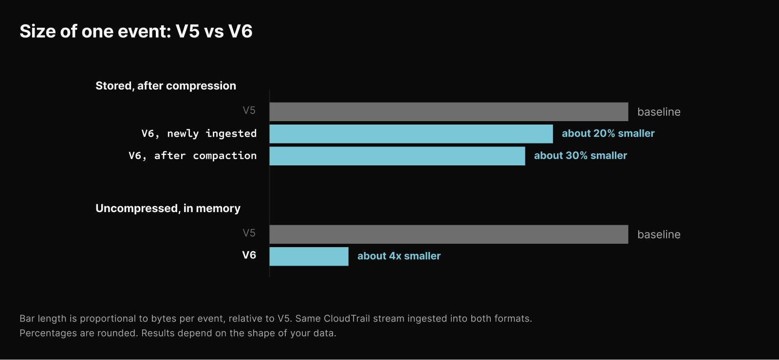
V6 stores about 25% fewer bytes per event (for typical logs), after compression. That's direct savings on your S3 bill. In our CloudTrail test, freshly ingested data was about 20% smaller, and data that had been compacted was closer to 30% smaller. Since most data ends up compacted, the larger number is the one that affects your S3 bill most at the end of the month.

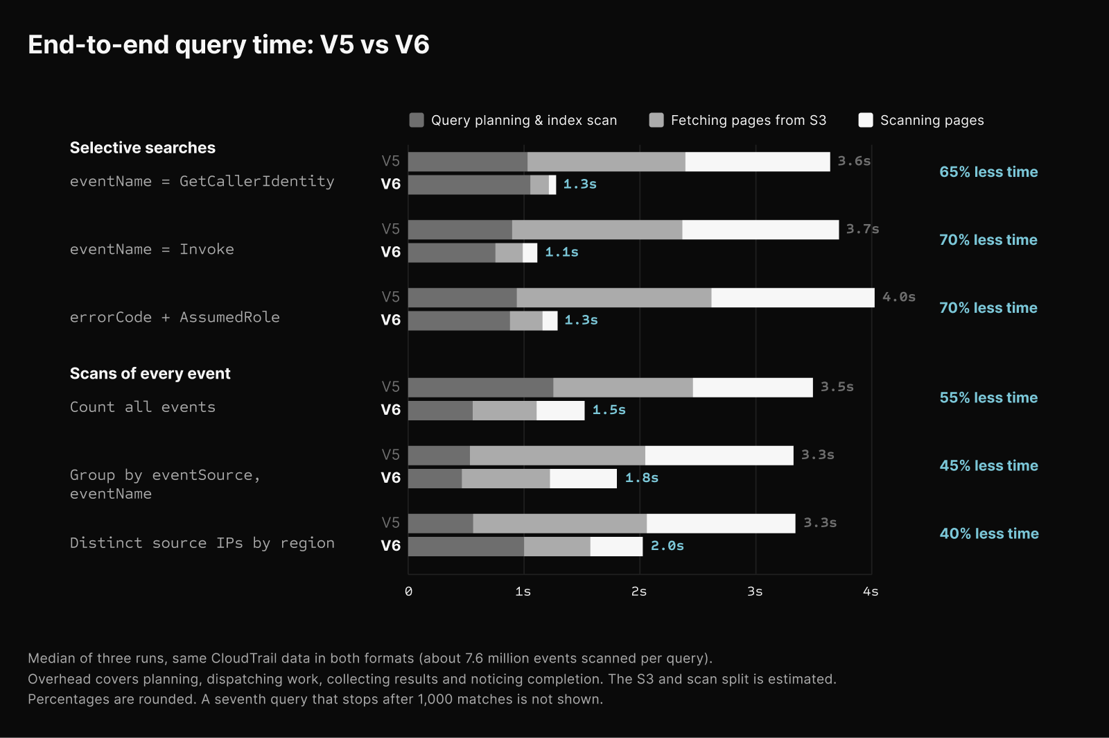
Fewer bytes also means less to fetch. Across our test queries, the time spent fetching pages from S3 dropped by 45-75%. Fetch time improved more than can be explained with just the smaller compressed footprint. We suspect that we're hitting bandwidth limits less often.

Once a page is loaded and decompressed, it's also much smaller in memory than a V5 page - around 4x smaller in our real-world testing. String deduplication is the star here.

Query speed

Queries finish 1.5-3x faster, end to end, measured from the moment the query is submitted to the moment it completes.

How much faster depends on the query. Selective searches, where the needle you're looking for is rare, get the most out of V6: they finish about 3x faster, because the columnar layout lets us skip nearly everything that isn't the needle. For these queries, the CPU time spent scanning pages drops by 6-10x. Aggregations over every event, where there's nothing to skip, finish about 2x faster, and scanning takes about half the compute.

Why are the end-to-end numbers smaller than the scan numbers? Every query has some fixed costs that don't depend on the storage format: planning the query, handing out work, collecting results, and noticing that everything is done. That adds up to about a second. The faster the scan, the bigger a share of the total that overhead becomes.

Ingest latency is unchanged. Newly-ingested data became searchable in just over a minute at the median in both formats.

Data compaction

Compaction is about twice as fast per event with V6. The biggest compactions benefit the most: in one test, the largest compaction went from a minute and a half to under half a minute.

The indexes we build alongside each data file got cheaper too, by about 10-30% depending on the index.

The encoding tradeoff

There is one cost here: encoding a page of data in the V6 format takes more work than in V5. This additional compute is the up-front cost of all the extra work that goes into the V6 format. That matters less than we expected. Encoding is one step in a pipeline that also parses, transforms, and writes the data, and in our test, the whole initial write step cost only a few percent more per event than it did with V5.

And there's a silver lining: everything that gets ingested gets compacted several times. In our test, the average event passed through compaction about three times. Since compactions are so much cheaper with V6, the small up-front cost is paid back quickly. Add up everything we do to an event over its lifetime, which is writing it, compacting it, and building its indexes, and V6 used about 25-30% less compute.

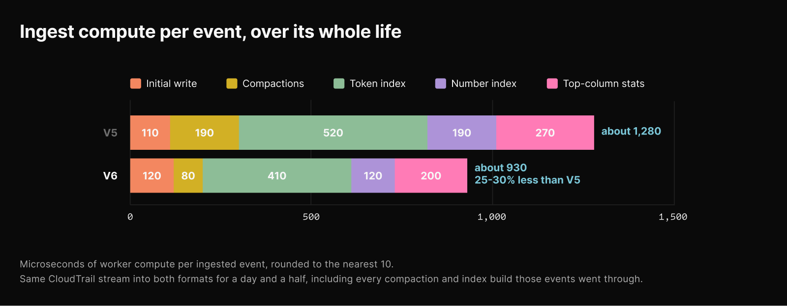
BYOC customers pay this compute directly; managed customers do not.

Rollout

With the rollout of V6, customers will see the benefits when querying newly-ingested data. Queries across different storage versions work seamlessly, without migrating your historical data.